The Wars Within Trump’s Court

via NYT > Top Stories https://ift.tt/BWfcXEN

They Were Waiting for Flights. Then Trump Closed a Door for Afghan Allies.

via NYT > Top Stories https://ift.tt/bWQLqcH

Federal Agencies Begin Removing DEI Guidance From Websites in Trump Crackdown

via TIME https://ift.tt/uMdTc70

Why Are the Oscars Scared of Horror Films?

via NYT > Top Stories https://ift.tt/9zndBHe

Federal Judge Temporarily Blocks Trump’s Executive Order Ending Birthright Citizenship

via TIME https://ift.tt/8P92CQo

OpenAI Unveils New Agent Tool ‘Operator’

via NYT > Top Stories https://ift.tt/N2dnMC1

‘The Return of the King’: Trump Embraces Trappings of the Throne

via NYT > Top Stories https://ift.tt/fywF4uK

Do Chimps Who Pee Together Stay Together?

via NYT > Top Stories https://ift.tt/h2ckiox

Loving an ‘Untouched’ Modernist House, and Then Getting Down to Work

via NYT > Top Stories https://ift.tt/Nfy7RBH

Louisiana Shuts 100-Mile Stretch of I-10 as Rare Snowstorm Hits Gulf Coast

via NYT > Top Stories https://ift.tt/wfPaJT8

 

Profit Margin Formula in Excel

 Calculating gross profit margin, operating profit margin and net profit margin in Excel is easy. Simply use the formulas explained on this page.

Gross Profit Margin

Assume your business had a total revenue of $10,000 in July and the cost of goods sold (COGS) equaled $4,000.

To calculate the gross profit margin, use the following formula:

Gross Profit Margin	=	Total Revenue - COGS
		Total Revenue

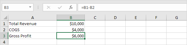
1. The formula below calculates the number above the fraction line. This is called the gross profit.

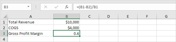
2. Divide this result by the total revenue to calculate the gross profit margin in Excel.

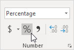
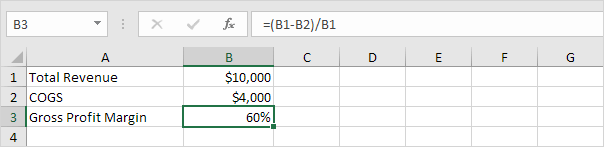
3. On the Home tab, click the percentage symbol to apply a Percentage format.

Result:

Operating Profit Margin

The operating profit margin also includes operating expenses (OPEX) such as rent, equipment, inventory costs, marketing, etc.

To calculate the operating profit margin, use the following formula:

Operating Profit Margin	=	Total Revenue - COGS - OPEX
		Total Revenue

1. The formula below calculates the number above the fraction line. This is called the operating profit.

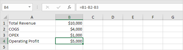
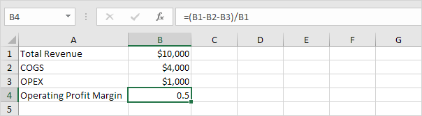
2. Divide this result by the total revenue to calculate the operating profit margin in Excel.

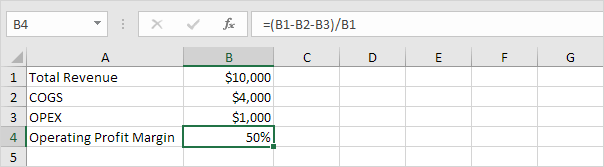
3. On the Home tab, click the percentage symbol to apply a Percentage format.

Result:

Net Profit Margin

The net profit margin also includes non-operating expenses such as interest (on debt) and taxes.

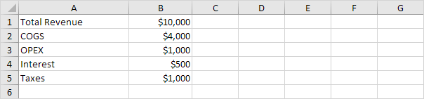
To calculate the net profit margin, use the following formula:

Net Profit Margin	=	Total Revenue - COGS - OPEX - I - T
		Total Revenue

where:

COGS = Cost of Goods Sold

OPEX = Operating expenses

I = Interest

T = Taxes

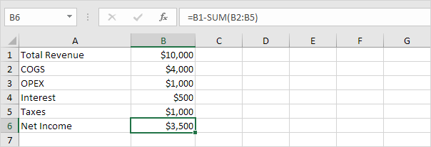
1. The formula below calculates the number above the fraction line. This is called the net income.

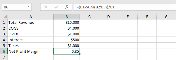
2. Divide this result by the total revenue to calculate the net profit margin in Excel.

3. On the Home tab, click the percentage symbol to apply a Percentage format.

Result:

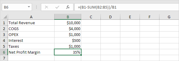
Conclusion: a 35% net profit margin means your business has a net income of $0.35 for each dollar of sales.

 

Depreciation Formulas in Excel

 

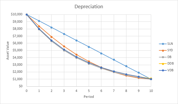
Excel offers five different depreciation functions. We consider an asset with an initial cost of $10,000, a salvage value (residual value) of $1000 and a useful life of 10 periods (years). Below you can find the results of all five functions. Each function will be explained separately in the next 5 paragraphs.

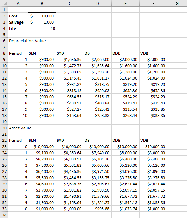
Most assets lose more value in the beginning of their useful life. The SYD, DB, DDB and VDB functions have this property.

SLN

The SLN (Straight Line) function is easy. Each year the depreciation value is the same.

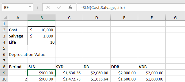
The SLN function performs the following calculation. Depreciation Value = (10,000 - 1,000) / 10 = 900.00. If we subtract this value 10 times, the asset depreciates from 10,000 to 1000 in 10 years (see first picture, bottom half).

SYD

The SYD (Sum of Years' Digits) function is also easy. As you can see below, this function also requires the period number.

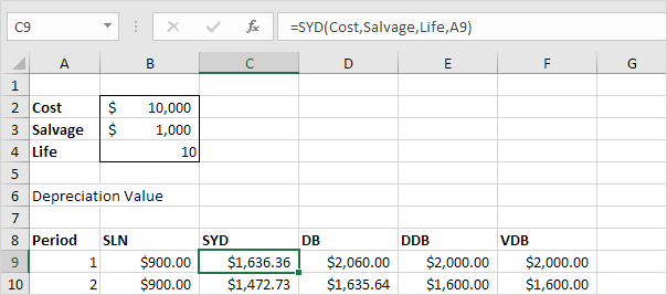
The SYD function performs the following calculations. A useful life of 10 years results in a sum of years of 10 + 9 + 8 + 7 + 6 + 5 + 4 + 3 + 2 + 1 = 55. The asset loses 9000 in value. Depreciation value period 1 = 10/55 * 9000 = 1,636.36. Depreciation value period 2 = 9/55 * 9000 = 1,472.73, etc. If we subtract these values, the asset depreciates from 10,000 to 1000 in 10 years (see first picture, bottom half).

DB

The DB (Declining Balance) function is a bit more complicated. It uses a fixed rate to calculate the depreciation values.

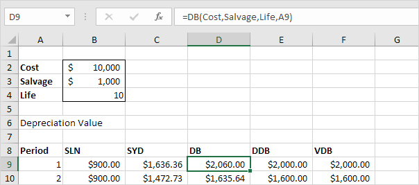
The DB function performs the following calculations. Fixed rate = 1 - ((salvage / cost) ^ (1 / life)) = 1 - (1000/10,000)^(1/10) = 1 - 0.7943282347 = 0.206 (rounded to 3 decimal places). Depreciation value period 1 = 10,000 * 0.206 = 2,060.00. Depreciation value period 2 = (10,000 - 2,060.00) * 0.206 = 1635.64, etc. If we subtract these values, the asset depreciates from 10,000 to 995.88 in 10 years (see first picture, bottom half).

Note: the DB function has a fifth optional argument. You can use this argument to indicate the number of months to go in the first year (If omitted, it is assumed to be 12). For example, set this argument to 9 if you purchase your asset at the beginning of the second quarter in year 1 (9 months to go in the first year). Excel uses a slightly different formula to calculate the depreciation value for the first and last period (the last period represents an 11th year with only 3 months).

DDB

The DDB (Double Declining Balance) function is easy again. However, sometimes you don't reach the salvage value when you use this function.

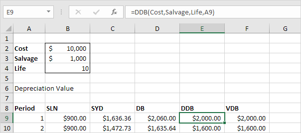
The DDB function performs the following calculations. A useful life of 10 years results in a rate of 1/10 = 0.1. Because this function is called Double Declining Balance we double this rate (factor = 2). Depreciation value period 1 = 10,000 * 0.2 = 2,000.00. Depreciation value period 2 = (10,000 - 2,000.00) * 0.2 = 1600.00, etc. As said earlier, sometimes you don't reach the salvage value when you use this function. In this example, if we subtract the depreciation values, the asset depreciates from 10,000 to 1073.74 in 10 years (see first picture, bottom half). However, read on to fix this.

Note: the DDB function has a fifth optional argument. You can use this argument to use a different factor.

VDB

The VDB (Variable Declining Balance) function uses the DDB (Double Declining Balance) method by default. The 4th argument indicates the starting period, the 5th argument indicates the ending period.

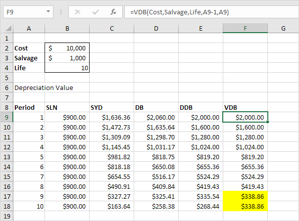
The VDB function performs the same calculations as the DDB function. However, it switches to Straight Line calculation (yellow values) to make sure you reach the salvage value (see first picture, bottom half). It only switches to Straight Line calculation when Depreciation Value, Straight Line is higher than Depreciation Value, DDB. In period 8, Depreciation Value, DDB = 419.43. We still have 2097.15 - 1000 (see first picture, bottom half) to depreciate. If we use the Straight Line method this results in 3 remaining depreciation values of 1097.15 / 3 = 365.72. Depreciation Value, Straight Line is not higher so we do not switch. In period 9, Depreciation Value, DDB = 335.54. We still have 1677.72 - 1000 (see first picture, bottom half) to depreciate. If we use Straight line method this results in 2 remaining depreciation values of 677.72 / 2 = 338.86. Depreciation Value, Straight Line is higher so we switch to Straight Line calculation.

Note: the VDB function is much more versatile than the DDB function. It can calculate the depreciation value of multiple periods. In this example, =VDB(Cost,Salvage,Life,0,3) reduces to 2000 + 1600 + 1280 = 4880. It contains a 6th and 7th optional argument. You can use the 6th argument to use a different factor. If you set the 7th argument to TRUE it does not switch to Straight Line calculation (the same as DDB).