CAGR formula in Excel

 

There's no CAGR function in Excel. However, simply use the RRI function in Excel to calculate the compound annual growth rate (CAGR) of an investment over a period of years.

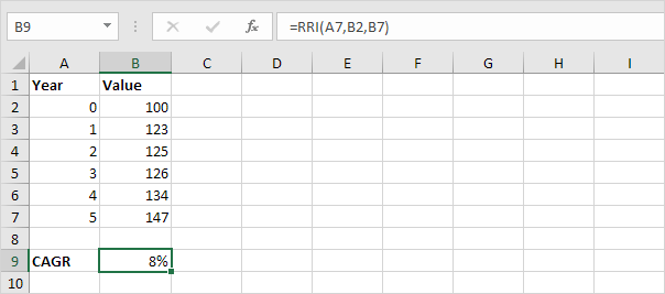
1. The RRI function below calculates the CAGR of an investment. The answer is 8%.

Note: the RRI function has three arguments (number of years = 5, start = 100, end = 147).

2. The CAGR measures the growth of an investment as if it had grown at a steady rate on an annually compounded basis. We can check this.

which is the same as:

Note: again, number of years or n = 5, start = 100, end = 147, CAGR = 8%.

3. Knowing this, we can easily create a CAGR formula that calculates the compound annual growth rate of an investment in Excel.

A2 = A1 * (1 + CAGR)ⁿ

end = start * (1 + CAGR)ⁿ

end/start = (1 + CAGR)ⁿ

(end/start)^1/n = (1 + CAGR)

CAGR = (end/start)^1/n - 1

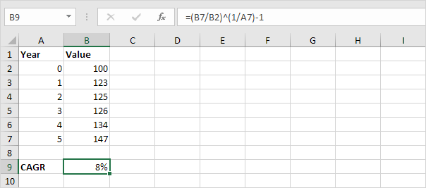
4. The CAGR formula below does the trick.

Note: in other words, to calculate the CAGR of an investment in Excel, divide the value of the investment at the end by the value of the investment at the start. Next, raise this result to the power of 1 divided by the number of years. Finally, subtract 1 from this result.

 

Compound Interest Formula in Excel

 What's compound interest and what's the formula for compound interest in Excel? This example gives you the answers to these questions.

1. Assume you put $100 into a bank. How much will your investment be worth after 1 year at an annual interest rate of 8%? The answer is $108.

2. Now this interest ($8) will also earn interest (compound interest) next year. How much will your investment be worth after 2 years at an annual interest rate of 8%? The answer is $116.64.

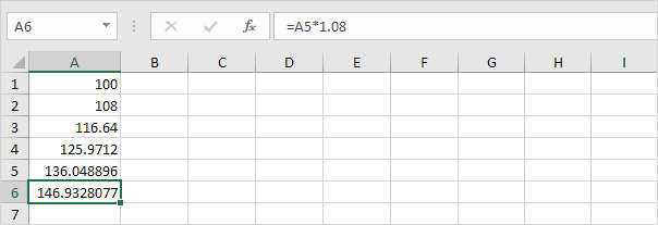
3. How much will your investment be worth after 5 years? Simply drag the formula down to cell A6.

The answer is $146.93.

4. All we did was multiplying 100 by 1.08, 5 times. So we can also directly calculate the value of the investment after 5 years.

which is the same as:

Note: there is no special function for compound interest in Excel. However, you can easily create a compound interest calculator to compare different rates and different durations.

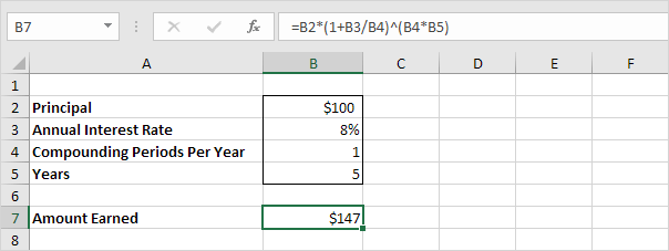
5. Assume you put $100 into a bank. How much will your investment be worth after 5 years at an annual interest rate of 8%? You already know the answer.

Note: the compound interest formula reduces to =100*(1+0.08/1)^(1*5), =100*(1.08)^5

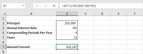
6. Assume you put $10,000 into a bank. How much will your investment be worth after 15 years at an annual interest rate of 4% compounded quarterly? The answer is $18,167.

Note: the compound interest formula reduces to =10000*(1+0.04/4)^(4*15), =10000*(1.01)^60

7. Assume you put $10,000 into a bank. How much will your investment be worth after 10 years at an annual interest rate of 5% compounded monthly? The answer is $16,470.

Note: the compound interest formula always works. If you're interested, download the Excel file and try it yourself!

 

Investment or Annuity in Excel

 This example teaches you how to calculate the future value of an investment or the present value of an annuity.

Tip: when working with financial functions in Excel, always ask yourself the question, am I making a payment (negative) or am I receiving money (positive)?

Investment

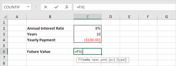
Assume that at the end of every year, you deposit $100 into a savings account. At an annual interest rate of 8%, how much will your investment be worth after 10 years?

1. Insert the FV (Future Value) function.

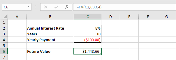
2. Enter the arguments.

In 10 years time, you pay 10 * $100 (negative) = $1000, and you'll receive $1,448.66 (positive) after 10 years. The higher the interest, the faster your money grows.

Note: the last two arguments are optional. If omitted, Pv = 0 (no present value). If Type is omitted, it is assumed that payments are due at the end of the period.

Annuity

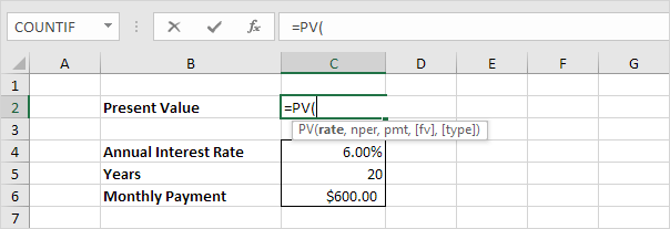
Assume you want to purchase an annuity that will pay $600 a month, for the next 20 years. At an annual interest rate of 6%, how much does the annuity cost?

1. Insert the PV (Present Value) function.

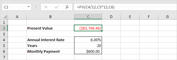
2. Enter the arguments.

You need a one-time payment of $83,748.46 (negative) to pay this annuity. You'll receive 240 * $600 (positive) = $144,000 in the future. This is another example that money grows over time.

Note: we receive monthly payments, so we use 6%/12 = 0.5% for Rate and 20*12 = 240 for Nper. The last two arguments are optional. If omitted, Fv = 0 (no future value). If Type is omitted, it is assumed that payments are due at the end of the period. This annuity does not take into account life expectancy, inflation etc.

Loans with Different Durations in Excel

 Loans with Different Durations in Excel

 

This example teaches you how to compare loans with different durations in Excel.

1. First, we calculate the monthly payment on a loan with an annual interest rate of 6%, a 20-year duration and a present value (amount borrowed) of $150,000.

Note: we make monthly payments, so we use 6%/12 = 0.5% for Rate and 20*12 = 240 for Nper (total number of periods).

2. Next, select the range A2:D2 and drag it down two rows.

3. Change the duration of the other two loans to 25 and 30 years.

Result:

The monthly payment over 30 years ($899.33) looks good in contrast to the $966.45 and $1,074.65. Right?

4. But now we calculate the Total Paid for each loan.

The monthly payment over 30 years ($899.33) suddenly does not look so attractive anymore. Conclusion: the longer the duration of the loan, the more interest you pay.

 

PMT function in Excel

 

The PMT function in Excel calculates the payment for a loan based on constant payments and a constant interest rate. This page contains many easy to follow PMT examples.

PMT examples

Consider a loan with an annual interest rate of 6%, a 20-year duration, a present value of $150,000 (amount borrowed) and a future value of 0 (that's what you hope to achieve when you pay off a loan).

1. The PMT function below calculates the annual payment.

Note: if the fifth argument is omitted, it is assumed that payments are due at the end of the period. We pay off a loan of $150,000 (positive, we received that amount) and we make annual payments of $13,077.68 (negative, we pay).

2. The PMT function below calculates the quarterly payment.

Note: we make quarterly payments, so we use 6%/4 = 1.5% for Rate and 20*4 = 80 for Nper (total number of periods).

3. The PMT function below calculates the monthly payment.

Note: we make monthly payments, so we use 6%/12 = 0.5% for Rate and 20*12 = 240 for Nper (total number of periods).

Consider an investment with an annual interest rate of 8% and a present value of 0. How much money should you deposit at the end of each year to have $1,448.66 in the account in 10 years?

4. The PMT function below calculates the annual deposit.

Explanation: in 10 years time, you pay 10 * $100 (negative) = $1000, and you'll receive $1,448.66 (positive) after 10 years. The higher the interest, the faster your money grows.

Consider an annuity with an annual interest rate of 6% and a present value of $83,748.46 (purchase value). How much money can you withdraw at the end of each month for the next 20 years?

5. The PMT function below calculates the monthly withdrawal.

Explanation: you need a one-time payment of $83,748.46 (negative) to pay this annuity. You'll receive 240 * $600 (positive) = $144,000 in the future. This is another example that money grows over time.

PPMT and IPMT

Consider a loan with an annual interest rate of 5%, a 2-year duration and a present value (amount borrowed) of $20,000.

1. The PMT function below calculates the monthly payment.

Note: we make monthly payments, so we use 5%/12 for Rate and 2*12 for Nper (total number of periods).

2. The PPMT function in Excel calculates the principal part of the payment. The second argument specifies the payment number.

Explanation: the PPMT function above calculates the principal part of the 5th payment.

3. The IPMT function in Excel calculates the interest part of the payment. The second argument specifies the payment number.

Explanation: the IPMT function above calculates the interest part of the 5th payment.

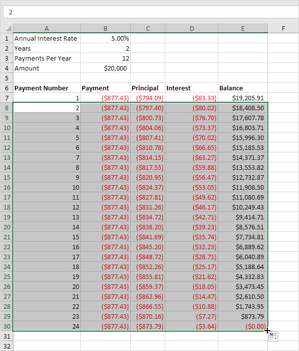
4. It takes 24 months to pay off this loan. Create a loan amortization schedule (see picture below) to clearly see how the principal part increases and the interest part decreases with each payment.

Note: the principal part and the interest part always add up to the payment amount.

Excel Regional Format Settings

 

Regional Format Settings

Excel provides regional formatting settings for different languages and styles of presenting information.

Regional settings affects a number of things, like:

• Calendar date formatting
• Decimal numbers
• Default currency formatting
• Formula delimiters

Formula delimiters are the symbols used to separate arguments in a function.

The most common symbols are comma , and semicolon ;

For example, the English regional language setting uses commas:

=AND([logical1], [logical2], ...)

Excel Format Grids

 

Grids

By default, gridlines are displayed in Excel.

However, grids can be removed.

Why remove grids?

• Make the spreadsheet more readable
• Make the spreadsheet more delicate

How to remove grids

1. Click view in the Ribbon navigation bar
2. Uncheck gridlines